

At Tines, we recently faced a significant engineering challenge: our output_payloads table in PostgreSQL was rapidly approaching 17TB on our largest cloud cluster, with no signs of slowing down. Once a table reaches PostgreSQL’s 32TB table size limit, it will stop accepting writes. This table holds event data, in the form of arbitrary JSON, which is critical to powering Tines workflows. Given the criticality of the data, we couldn’t risk any disruptions to it.
As our monitoring showed the table's growth, we began experiencing warning signs. Cleanup jobs on the table had begun to time out. The table was causing increased I/O pressure on our infrastructure, leading us to use more expensive hardware. The arbitrary JSON shape of the data meant massive autovacuum jobs on its TOAST table. When these autovacuums ran, they displaced other tables from the buffer cache, forcing disk reads in critical areas. As a bandaid, we modified the autovacuum parameters of the table so that the autovacuums would run more frequently, but have less tuples to process. With performance slowly degrading, and 32TB looming on the horizon, we knew we needed to act decisively.
Enter: Partitioning
We started off with partitioning over sharding, which involves splitting data across multiple independent database instances. We took this approach as we wanted to avoid the complexities of sharding until we were convinced it was absolutely necessary.
To partition a database table is to divide it into multiple, smaller tables. Each of these smaller tables is a sub-table of the main table, and therefore holds a subset of the data that belongs to the main table. Partitioning is a good idea when you want to spread the data in one table to many tables for better query performance. With partitioning, the database needs to scan less data for each query. Tables that are ideal candidates for partitioning typically exhibit characteristics like: substantial size, high data ingestion rates, significant maintenance overhead (such as prolonged vacuuming and indexing operations), and noticeable query performance degradation. We started to observe these characteristics on our output_payloads table. You can’t alter an existing table to be a partitioned one without taking a downtime, however, so we would have to start fresh with a new, partitioned table. We named the the new table event_payloads.
Our quest for the optimal partitioning strategy
We ingest over 6TB of data daily in our cloud clusters. This volume made it essential that we select a partitioning strategy capable of efficiently handling our two most important query patterns: point queries and range queries. Point queries find specific records by their unique identifiers and/or attributes, such as by id, while range queries retrieve sets of records where a specific value falls within a defined upper and lower boundary. An example of a common range query is time periods, such as querying for all records created within the last 24 hours. As much as possible, we knew we’d need to ensure even data distribution across partitions to prevent what we called "hot partitions," where a disproportionate amount of rows concentrate in specific partitions. Such imbalances could cause tasks like autovacuum to time out as a single partition grows, and force point queries to scan excessive amounts of data. The goal was to maintain consistent performance, while accommodating our massive data ingestion requirements. In our quest for the optimal partitioning strategy, we considered four different approaches:
Strategy 1: Partition based on created_at
With this strategy, we would partition the data such that records created on the same day would be stored in a single table. For example, the sub-tables would look like:
event_payloads_p2025_03_21  -- Contains all records from March 21, 2025
event_payloads_p2025_03_22  -- Contains all records from March 22, 2025
event_payloads_p2025_03_23  -- Contains all records from March 23, 2025
A time-based partitioning strategy like this works well for cleaning up expired data. In our app, users can choose how long to keep their data for (up to a year). With time-based partitioning, that meant we could safely drop an entire partition after a year. In order to drop old partitions and create new ones on a schedule, we could use a ruby gem called pg_partition_manager. This gem simplifies the management of partitioned tables in PostgreSQL by programmatically creating new partitions and dropping old ones as data ages out. Although it sounded promising, time-based partitioning complicated point queries. There are several places in our app where we query for event_payloads by id and/or some other specific value. With this strategy, PostgreSQL had no way of knowing which partition contained the target records. Therefore, it had to scan every partition until it found the event_payload(s) with the specified values.
Here is an example query that we might have in our app:
SELECT * FROM event_payloads
WHERE id IN (1088692569,1088694904,1088696787,1089012063,1089012074) AND key = 'get_alert_details';
This was the query plan partitioning by day (truncated):
Limit  (cost=207.43..207.48 rows=22 width=125) (actual time=0.148..0.155 rows=0 loops=1)
  Buffers: shared hit=44
  ->  Sort  (cost=207.43..207.48 rows=22 width=125) (actual time=0.147..0.153 rows=0 loops=1)
        Sort Key: event_payloads.id DESC
        Sort Method: quicksort  Memory: 25kB
        Buffers: shared hit=44
        ->  Append  (cost=0.29..206.94 rows=22 width=125) (actual time=0.141..0.147 rows=0 loops=1)
              Buffers: shared hit=44
              ->  Index Scan using event_payloads_p2025_03_21_tenant_id_idx on event_payloads_p2025_03_21 event_payloads_1  (cost=0.29..4.32 rows=1 width=202) (actual time=0.025..0.025 rows=0 loops=1)
                    Index Cond: (tenant_id = 24020)
                    Filter: (((key)::text = 'get_alert_details'::text) AND (id = ANY ('{1088692569,1088694904,1088696787,1089012063,1089012074}'::bigint[])))
                    Buffers: shared hit=2
              ->  Index Scan using event_payloads_p2025_03_22_tenant_id_idx on event_payloads_p2025_03_22 event_payloads_2  (cost=0.29..4.32 rows=1 width=202) (actual time=0.015..0.015 rows=0 loops=1)
                    Index Cond: (tenant_id = 24020)
                    Filter: (((key)::text = 'get_alert_details'::text) AND (id = ANY ('{1088692569,1088694904,1088696787,1089012063,1089012074}'::bigint[])))
                    Buffers: shared hit=2
              ->  Index Scan using event_payloads_p2025_03_23_tenant_id_idx on event_payloads_p2025_03_23 event_payloads_3  (cost=0.29..4.32 rows=1 width=202) (actual time=0.016..0.016 rows=0 loops=1)
                    Index Cond: (tenant_id = 24020)
                    Filter: (((key)::text = 'get_alert_details'::text) AND (id = ANY ('{1088692569,1088694904,1088696787,1089012063,1089012074}'::bigint[])))
                    Buffers: shared hit=2
....
              ->  Bitmap Heap Scan on event_payloads_p2025_03_26 event_payloads_6  (cost=4.17..11.31 rows=1 width=96) (actual time=0.005..0.005 rows=0 loops=1)
                    Recheck Cond: (tenant_id = 24020)
                    Filter: (((key)::text = 'get_alert_details'::text) AND (id = ANY ('{1088692569,1088694904,1088696787,1089012063,1089012074}'::bigint[])))
                    Buffers: shared hit=2
                    ->  Bitmap Index Scan on event_payloads_p2025_03_26_tenant_id_idx  (cost=0.00..4.17 rows=3 width=0) (actual time=0.003..0.003 rows=0 loops=1)
                          Index Cond: (tenant_id = 24020)
                          Buffers: shared hit=2
              ->  Bitmap Heap Scan on event_payloads_p2025_03_27 event_payloads_7  (cost=4.17..11.31 rows=1 width=96) (actual time=0.002..0.003 rows=0 loops=1)
                    Recheck Cond: (tenant_id = 24020)
                    Filter: (((key)::text = 'get_alert_details'::text) AND (id = ANY ('{1088692569,1088694904,1088696787,1089012063,1089012074}'::bigint[])))
                    Buffers: shared hit=2
                    ->  Bitmap Index Scan on event_payloads_p2025_03_27_tenant_id_idx  (cost=0.00..4.17 rows=3 width=0) (actual time=0.002..0.002 rows=0 loops=1)
                          Index Cond: (tenant_id = 24020)
                          Buffers: shared hit=2
              ->  Bitmap Heap Scan on event_payloads_p2025_03_28 event_payloads_8  (cost=4.17..11.31 rows=1 width=96) (actual time=0.002..0.002 rows=0 loops=1)
                    Recheck Cond: (tenant_id = 24020)
                    Filter: (((key)::text = 'get_alert_details'::text) AND (id = ANY ('{1088692569,1088694904,1088696787,1089012063,1089012074}'::bigint[])))
                    Buffers: shared hit=2
                    ->  Bitmap Index Scan on event_payloads_p2025_03_28_tenant_id_idx  (cost=0.00..4.17 rows=3 width=0) (actual time=0.002..0.002 rows=0 loops=1)
                          Index Cond: (tenant_id = 24020)
                          Buffers: shared hit=2
....


Planning:
  Buffers: shared hit=32
Planning Time: 1.137 ms
Execution Time: 5.559 ms
The query planner couldn't do any partition pruning because we couldn't filter by created_at. Partition pruning works by only searching partitions that can contain records of interest, but since our records of interest could have been created on any day, all partitions had to be searched. The scanning of every partition led to unacceptably high CPU, so we ruled this strategy out.
Strategy 2: Partition based on root_story_id
In our app, each of these event_payloads gets created within a “story”. It’s a one-to-many relationship, with each story having many event_payloads, but each event_payload belonging to only one story, which can be identified by its root_story_id. The idea with this strategy was to have a fixed number of partitions and use PostgreSQL’s hash-based partitioning.
We chose 16 tables, and the creation of these tables looked like this:
   def self.create_partitioned_tables
      # Create the parent table with first-level partitioning on root_story_id
      sql = <<~SQL
        CREATE TABLE IF NOT EXISTS event_payloads (
          id BIGSERIAL NOT NULL,
          key CHARACTER VARYING NOT NULL,
          output JSON,
          tenant_id BIGINT NOT NULL,
          root_story_id BIGINT NOT NULL,
          created_at TIMESTAMP WITHOUT TIME ZONE NOT NULL,
          updated_at TIMESTAMP WITHOUT TIME ZONE NOT NULL,
          PRIMARY KEY (root_story_id, id)
        ) PARTITION BY HASH (root_story_id);
      SQL

      # Create 16 partitions for partitioning by root_story_id
      (0..15).each do |i|
        sql += <<~SQL
          CREATE TABLE event_payloads_#{i} PARTITION OF event_payloads
            FOR VALUES WITH (modulus 16, remainder #{i});
        SQL
      end

      sql += <<~SQL
        CREATE INDEX IF NOT EXISTS index_event_payloads_on_tenant_id ON event_payloads(tenant_id);
      SQL

      ActiveRecord::Base.connection.execute(sql)
    end
After PostgreSQL applied its own hash function to the root_story_id, the hashed value would determine where the event_payloads for that story would be stored. For example, if the hashed value for a root_story_id, modulo 16, was 2, records for that story would be stored in event_payloads_2. While it made sense to have all of the data for a story in the same partition, this would create the “hot partitions” we were trying to avoid. A few busy stories creating a lot of event_payloads would disproportionately ingest data into their respective partitions, and the size of those tables would grow much faster relative to other tables getting populated by less busy stories. We passed on this strategy in the interest of more even data distribution.
Strategy 3: Partition based on id, with an index on root_story_id
This approach used the same hash-based partitioning technique as described in Strategy 2, but instead of hashing the root_story_id, we hashed the id of the event_payload itself. The index on root_story_id would come in handy because anywhere we query for events in our app, we know what story we are interested in, so we could use a WHERE clause to filter for a certain root_story_id.
CREATE TABLE event_payloads (
  id bigserial,
  key text NOT NULL,
  output jsonb,
  created_at timestamp NOT NULL,
  updated_at timestamp NOT NULL,
  root_story_id bigint NOT NULL,
  PRIMARY KEY (id, root_story_id)
) PARTITION BY HASH (id);

CREATE TABLE event_payloads_0 PARTITION OF event_payloads
  FOR VALUES WITH (modulus 4, remainder 0);
CREATE TABLE event_payloads_1 PARTITION OF event_payloads
  FOR VALUES WITH (modulus 4, remainder 1);
CREATE TABLE event_payloads_2 PARTITION OF event_payloads
  FOR VALUES WITH (modulus 4, remainder 2);
CREATE TABLE event_payloads_3 PARTITION OF event_payloads
  FOR VALUES WITH (modulus 4, remainder 3);

CREATE INDEX idx_event_payloads_root_story_id ON event_payloads(root_story_id);
This approach ensured even data distribution because where an event_payload ended up wasn’t dependent on the context it was created in at all. Therefore, the “hot partition” problem was eliminated.
Point queries searching for just one, or multiple, specific event_payload(s) by id(s) were extremely efficient, immediately searching the partition containing the event_payload(s) in question:
EXPLAIN ANALYZE
SELECT * FROM event_payloads
WHERE id = 1234 AND root_story_id = 100;

Index Scan using event_payloads_2_pkey on event_payloads_2 event_payloads  (cost=0.28..8.30 rows=1 width=64) (actual time=0.016..0.017 rows=1 loops=1)
  Index Cond: ((id = 1234) AND (root_story_id = 100))
Planning Time: 0.340 ms
Execution Time: 0.039 ms
Querying for all event_payloads in a story forced a scan of all partitions, but the index on root_story_id was used effectively:
EXPLAIN ANALYZE
SELECT * FROM event_payloads
WHERE root_story_id = 100;

Append  (cost=0.15..66.11 rows=1000 width=64) (actual time=0.014..0.218 rows=1000 loops=1)
  ->  Index Scan using event_payloads_0_root_story_id_idx on event_payloads_0 event_payloads_1  (cost=0.15..14.32 rows=238 width=64) (actual time=0.013..0.045 rows=238 loops=1)
        Index Cond: (root_story_id = 100)
  ->  Index Scan using event_payloads_1_root_story_id_idx on event_payloads_1 event_payloads_2  (cost=0.15..15.82 rows=267 width=64) (actual time=0.008..0.042 rows=267 loops=1)
        Index Cond: (root_story_id = 100)
  ->  Index Scan using event_payloads_2_root_story_id_idx on event_payloads_2 event_payloads_3  (cost=0.15..15.63 rows=256 width=64) (actual time=0.007..0.039 rows=256 loops=1)
        Index Cond: (root_story_id = 100)
  ->  Index Scan using event_payloads_3_root_story_id_idx on event_payloads_3 event_payloads_4  (cost=0.15..15.34 rows=239 width=64) (actual time=0.007..0.035 rows=239 loops=1)
        Index Cond: (root_story_id = 100)
Planning Time: 0.409 ms
Execution Time: 0.284 ms
However, range queries, particularly ones used for expiring records based on created_at were inefficient, so we decided to pass on this approach.
Strategy 4: Two-level partitioning by root_story_id and id
The idea with this approach was to strike a balance between optimal data distribution and efficient queries. The first level of partitions hashed by root_story_id as described in Strategy 2, but within each of those partitions, we introduced a second level of partitions, hashed by the id of the record itself as described in Strategy 3. Therefore, we had 128 partitions created like so:
    def self.create_partitioned_tables
      # Create the parent table with first-level partitioning on root_story_id
      sql = <<~SQL
        CREATE TABLE IF NOT EXISTS event_payloads (
          id BIGSERIAL NOT NULL,
          key CHARACTER VARYING NOT NULL,
          output JSON,
          tenant_id BIGINT NOT NULL,
          root_story_id BIGINT NOT NULL,
          created_at TIMESTAMP WITHOUT TIME ZONE NOT NULL,
          updated_at TIMESTAMP WITHOUT TIME ZONE NOT NULL,
          PRIMARY KEY (root_story_id, id)
        ) PARTITION BY HASH (root_story_id);
      SQL

      # Create 16 first-level partitions for partitioning by root_story_id, each sub-partitioned by id
      (0..15).each do |i|
        sql += <<~SQL
          CREATE TABLE event_payloads_#{i} PARTITION OF event_payloads
            FOR VALUES WITH (modulus 16, remainder #{i})
            PARTITION BY HASH (id);
        SQL

        # Create 8 sub-partitions for each first-level partition, partitioning by id
        (0..7).each { |j| sql += <<~SQL }
            CREATE TABLE event_payloads_#{i}_#{j} PARTITION OF event_payloads_#{i}
              FOR VALUES WITH (modulus 8, remainder #{j});
          SQL
      end

      sql += <<~SQL
        CREATE INDEX IF NOT EXISTS index_event_payloads_on_tenant_id ON event_payloads(tenant_id);
      SQL

      ActiveRecord::Base.connection.execute(sql)
    end
This gave us the benefit of not having to scan all partitions when looking for all records belonging to a story (only 8/128 as opposed to 4/4), but also distributed the event_payloads for any one story across eight partitions, mitigating the “hot partition” problem.
Point queries searching for specific id(s) using the root_story_id were extremely efficient, searching only the partitions that contained the records we were looking for:
SELECT * FROM event_payloads
WHERE id IN (54472978, 177425082) AND root_story_id = 238;

 Append  (cost=0.42..25.77 rows=2 width=479) (actual time=0.027..0.051 rows=2 loops=1)
   ->  Index Scan using event_payloads_0_2_pkey on event_payloads_0_2 event_payloads_1  (cost=0.42..12.88 rows=1 width=480) (actual time=0.026..0.032 rows=1 loops=1)
         Index Cond: ((root_story_id = 238) AND (id = ANY ('{54472978,177425082}'::bigint[])))
   ->  Index Scan using event_payloads_0_5_pkey on event_payloads_0_5 event_payloads_2  (cost=0.42..12.88 rows=1 width=478) (actual time=0.017..0.017 rows=1 loops=1)
         Index Cond: ((root_story_id = 238) AND (id = ANY ('{54472978,177425082}'::bigint[])))
 Planning Time: 0.306 ms
 Execution Time: 0.098 ms
(7 rows)
Queries looking for all records belonging to a story were also efficient, because partition pruning made it so that only eight top-level partitions had to be searched:
SELECT * FROM event_payloads
WHERE root_story_id = 238;

 Append  (cost=0.00..469871.09 rows=2298420 width=480) (actual time=0.006..4744.669 rows=2415908 loops=1)
   ->  Seq Scan on event_payloads_0_0 event_payloads_1  (cost=0.00..57293.60 rows=287234 width=483) (actual time=0.005..491.770 rows=301253 loops=1)
         Filter: (root_story_id = 238)
         Rows Removed by Filter: 304997
   ->  Seq Scan on event_payloads_0_1 event_payloads_2  (cost=0.00..57213.86 rows=286518 width=483) (actual time=0.164..560.221 rows=301676 loops=1)
         Filter: (root_story_id = 238)
         Rows Removed by Filter: 304120
   ->  Seq Scan on event_payloads_0_2 event_payloads_3  (cost=0.00..57381.71 rows=290054 width=480) (actual time=0.175..552.702 rows=302427 loops=1)
         Filter: (root_story_id = 238)
         Rows Removed by Filter: 305111
   ->  Seq Scan on event_payloads_0_3 event_payloads_4  (cost=0.00..57296.16 rows=285988 width=478) (actual time=0.153..581.496 rows=301111 loops=1)
         Filter: (root_story_id = 238)
         Rows Removed by Filter: 303883
   ->  Seq Scan on event_payloads_0_4 event_payloads_5  (cost=0.00..57296.96 rows=289212 width=480) (actual time=0.178..573.105 rows=302489 loops=1)
         Filter: (root_story_id = 238)
         Rows Removed by Filter: 304290
   ->  Seq Scan on event_payloads_0_5 event_payloads_6  (cost=0.00..57354.15 rows=284877 width=478) (actual time=0.159..571.096 rows=302068 loops=1)
         Filter: (root_story_id = 238)
         Rows Removed by Filter: 305836
   ->  Seq Scan on event_payloads_0_6 event_payloads_7  (cost=0.00..57265.78 rows=284224 width=480) (actual time=0.149..595.128 rows=302069 loops=1)
         Filter: (root_story_id = 238)
         Rows Removed by Filter: 304993
   ->  Seq Scan on event_payloads_0_7 event_payloads_8  (cost=0.00..57276.76 rows=290313 width=479) (actual time=0.173..626.301 rows=302815 loops=1)
         Filter: (root_story_id = 238)
         Rows Removed by Filter: 303950
 Planning Time: 2.565 ms
 Execution Time: 4848.421 ms
(27 rows)
We concluded that this strategy provided the benefits that we found with the other strategies, while mitigating the shortcomings. It would scale well on both our multi-tenant clusters, where query efficiency is key, and our single-tenant clusters, where we risked a few busy stories creating “hot partitions”. In order to solve the problem of inefficient range queries, we eliminated the need to filter by created_at at all when cleaning up event_payload records. Instead of expiring event_payloads after their associated event was deleted, we pivoted towards deleting them inline with their event like so:
        query = <<~SQL
          DELETE FROM events
          WHERE id = ANY(ARRAY[:ids_to_delete])
          RETURNING event_payload_id
        SQL

        sanitized_query =
          ActiveRecord::Base.sanitize_sql_array([query, { ids_to_delete: batch.map(&:id) }])
        result = ApplicationRecord.execute_write_query(sanitized_query).to_a

        event_payload_ids = result.filter_map { |row| row["event_payload_id"] }

        if event_payload_ids.any?
          EventPayload.delete_by_ids(event_payload_ids, story.live_root_story_id)
        end
The journey
Deciding on a partitioning strategy was just the beginning of this project. Next, we set up the partitions as described in Strategy 4 on a test cluster. With the partitions in place, our general approach was to deploy code that relied on the event_payloads table everywhere we currently used the output_payloads table, load test, analyze performance, make adjustments, repeat. Load testing meant running a few busy stories on the test cluster, generating tons of writes and reads on the table. We tracked the performance in AWS Aurora/RDS console, identifying queries that caused high database load. We used PostgreSQL’s EXPLAIN ANALYZE tool in order to see how PostgreSQL was planning and executing resource intensive queries. From there, we could look for ways to optimize.
One thing that became apparent very early was that every query would have to have a WHERE clause on root_story_id in order to force index scans.
For example:
EXPLAIN ANALYZE
SELECT "event_payloads".*
FROM "event_payloads"
WHERE "event_payloads"."tenant_id" = 1
  AND "event_payloads"."id" = 14
LIMIT 1;

 Limit  (cost=0.42..12046.56 rows=1 width=587) (actual time=95.242..95.248 rows=1 loops=1)
   ->  Append  (cost=0.42..192738.51 rows=16 width=587) (actual time=95.241..95.247 rows=1 loops=1)
         ->  Index Scan using event_payloads_0_0_pkey on event_payloads_0_0 event_payloads_1  (cost=0.42..17027.20 rows=1 width=483) (actual time=11.138..11.138 rows=0 loops=1)
               Index Cond: (id = 14)
               Filter: (tenant_id = 1)
         ->  Index Scan using event_payloads_1_0_pkey on event_payloads_1_0 event_payloads_2  (cost=0.41..9689.27 rows=1 width=762) (actual time=0.403..0.403 rows=0 loops=1)
               Index Cond: (id = 14)
               Filter: (tenant_id = 1)
         ->  Index Scan using event_payloads_2_0_pkey on event_payloads_2_0 event_payloads_3  (cost=0.42..7860.12 rows=1 width=604) (actual time=1.350..1.350 rows=0 loops=1)
               Index Cond: (id = 14)
               Filter: (tenant_id = 1)
         ->  Index Scan using event_payloads_3_0_pkey on event_payloads_3_0 event_payloads_4  (cost=0.41..5262.14 rows=1 width=564) (actual time=0.766..0.766 rows=0 loops=1)
               Index Cond: (id = 14)
               Filter: (tenant_id = 1)
         ->  Index Scan using event_payloads_4_0_pkey on event_payloads_4_0 event_payloads_5  (cost=0.41..4020.52 rows=1 width=333) (actual time=0.257..0.257 rows=0 loops=1)
               Index Cond: (id = 14)
               Filter: (tenant_id = 1)
         ->  Index Scan using event_payloads_5_0_pkey on event_payloads_5_0 event_payloads_6  (cost=0.43..65567.71 rows=1 width=453) (actual time=42.546..42.546 rows=0 loops=1)
               Index Cond: (id = 14)
               Filter: (tenant_id = 1)
         ->  Index Scan using event_payloads_6_0_pkey on event_payloads_6_0 event_payloads_7  (cost=0.42..6771.96 rows=1 width=572) (actual time=2.209..2.210 rows=0 loops=1)
               Index Cond: (id = 14)
               Filter: (tenant_id = 1)
         ->  Index Scan using event_payloads_7_0_pkey on event_payloads_7_0 event_payloads_8  (cost=0.42..15250.86 rows=1 width=1204) (actual time=7.273..7.273 rows=0 loops=1)
               Index Cond: (id = 14)
               Filter: (tenant_id = 1)
         ->  Index Scan using event_payloads_8_0_pkey on event_payloads_8_0 event_payloads_9  (cost=0.41..4228.43 rows=1 width=485) (actual time=1.094..1.094 rows=0 loops=1)
               Index Cond: (id = 14)
               Filter: (tenant_id = 1)
         ....
         ....
 Planning Time: 0.766 ms
 Execution Time: 95.379 ms
(52 rows)
Vs. also filtering for root_story_id:
EXPLAIN ANALYZE
SELECT "event_payloads".*
FROM "event_payloads"
WHERE "event_payloads"."tenant_id" = 1
AND "event_payloads"."id" = 14
AND "event_payloads"."root_story_id" = 5779
LIMIT 1;
Limit (cost=0.42..8.44 rows=1 width=628) (actual time=0.020..0.020 rows=1 loops=1)
-> Index Scan using event_payloads_15_0_pkey on event_payloads_15_0 event_payloads (cost=0.42..8.44 rows=1 width=628) (actual time=0.019..0.019 rows=1 loops=1)
Index Cond: ((root_story_id = 5779) AND (id = 14))
Filter: (tenant_id = 1)
Planning Time: 0.168 ms
Execution Time: 0.041 ms
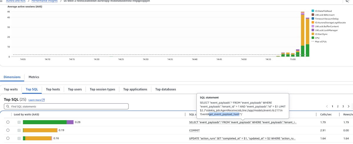
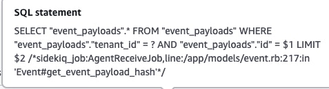
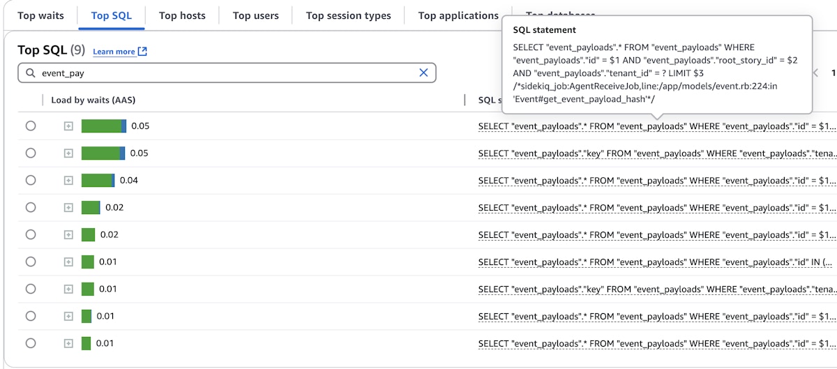
(6 rows)Here is another example where you can see the difference in database load by adding a filter on root_story_id, all other things kept the same:
Filtering for root_story_id helped to optimize SELECT queries, but they still didn’t perform as well as equivalent queries to the old table. A goal of this project was no regression from current behavior or performance, so we had some problem solving to do.
The queries on the event_payloads table were still causing higher CPU, and were less efficient than on the output_payloads table. This was because of what happens in PostgreSQL when you query partitions through the parent table. PostgreSQL must perform catalog lookups, particularly using pg_class and pg_inherits, and also perform its own hash calculation, to route each query to the correct partition. This results in significant overhead when you’re querying the table a lot, especially if you decide to use multi-level partitioning schemes like we did, where PostgreSQL must query the PostgreSQL catalog tables to identify the target partition. We do over 1 billion action runs a week in cloud, and this is one of the highest read code paths, so safe to say we’re querying this table a lot. For example, when we were doing something like:
SELECT
  "event_payloads".*
FROM
  "event_payloads"
WHERE
  "event_payloads"."tenant_id" = 1
  AND "event_payloads"."id" = 14
  AND "event_payloads"."root_story_id" = 5779;
PostgresSQL had to do a catalog lookup to figure out which child partition of the event_payloads table that particular record belongs to. This catalog lookup added overhead, and made the query more CPU intensive (which also largely came from the hash calculation for the partition key) and slower, as opposed to querying a non-partitioned table.
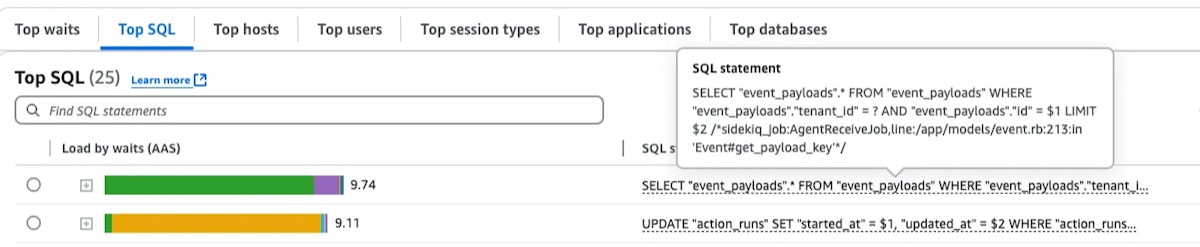
In order to mitigate this issue, we reverse engineered the PostgreSQL hash-based partitioning logic so that we could derive which partition an event_payload record would be in and query that partition directly. More specifically, this required replicating the logic of PostgreSQL’s hashint8extended function, which takes a value for the partition key, and a constant “seed” value defined by PostgreSQL in order to determine the integer that the key value hashes to. For example, if an event_payload had a root_story_id of 63, and an id of 244, we could use those two values to determine which of the first level partitions that root_story_id hashed to, and which second level partition that id hashed to. Therefore, we could build the name of the partition, something like event_payloads_11_1. This method of querying the partitions directly was 20-40x faster than their equivalent query relying on PostgreSQL’s catalog lookup.
Before reverse engineering PostgreSQL’s hash function:
Vs. the control (old output_payloads table):
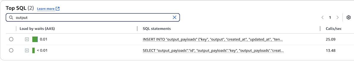
Vs. after reverse engineering (notice no SELECTs on event_payloads generated enough load to be displayed anymore):
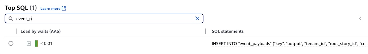
In order to make use of our ability to determine which partition event_payloads would be stored in, we defined our own event_payload function to override the default rails event.event_payload. Our function uses the event_payload_id of the event and our reverse engineered PostgreSQL hash function to query the event_payload’s partition for the record directly:
  sig { returns(T.nilable(EventPayload)) }
  def event_payload
    return unless event_payload_id.present? && story.present?

    EventPayload.from_partition(T.must(story).live_root_story_id, [T.must(event_payload_id)]).first
  end
This from_partition function uses the following helpers in order to derive the partition:
  sig { params(root_story_id: Integer).returns(String) }
  def self.root_story_partition_name(root_story_id)
    root_story_partition =
      PgHashFunc.calculate_partition_index_bigint(
        value: root_story_id,
        num_partitions: NUM_FIRST_LEVEL_PARTITIONS,
      )
    [TABLE_PREFIX, root_story_partition].join("_")
  end

  sig { params(root_story_id: Integer, ids: T::Array[Integer]).returns(String) }
  def self.partition_name(root_story_id, ids = [])
    root_story_partition = root_story_partition_name(root_story_id) # this gets us something like "event_payloads_0"
    return root_story_partition if ids.size != 1

    event_payload_partition =
      PgHashFunc.calculate_partition_index_bigint(
        value: ids.first,
        num_partitions: NUM_SECOND_LEVEL_PARTITIONS,
      )
    [root_story_partition, event_payload_partition].join("_") # then this gets us to something like "event_payloads_0_0"
  end
Rollout
The phases of rollout for this project, all controlled by different feature flags, were:
Dual writes: writing to both the new table and the old table at the same time
Verification: reading from the new table to verify data consistency between the old table and the new table, while still relying on the old table
Reading from the new table primarily, with fall back to the old table when the new table didn’t return any data
Dual writes
Dual writes was pretty straightforward to roll out. It required flipping on a feature flag and thereby starting to write equivalent records to both the old table and the new table for each event.
Verification
The dual reads (or shadow reads) phase of the rollout meant that we were also querying the new table everywhere we queried the old table. This was our time to verify that the new table was returning the same data as the old table, and could therefore be trusted as the primary read. In order to compare the data returned from the two tables, we used a Ruby library called Github scientist. This library is designed as an aid for refactoring critical code paths. With Github scientist, you can set up “experiments” where your application primarily uses the old method, while trying the new method. The library reports whether or not the two methods matched, which was data we could send to our monitoring system, Honeycomb. Github scientist also allows you to log any relevant metadata, which in our case were things like the event_id, the event_payload_id, and the output_payload_id. That way, we could go into Rails console and debug mismatches by looking at the records. For this project, we were concerned with the output field of event_payload records matching the output field of their corresponding output_payload record for any given event. The output field contains the arbitrary JSON that forms the core content of an event, so we needed to be sure we were getting the right data.
For the most part, the mismatches that we saw were expected. These were events created before we turned on dual writes, which wouldn't have an event_payload (i.e., the event_payload_id field was null). There were some unexpected mismatches on new event data, however, which required a closer look at those events and the way that they were created.
Once we were seeing near 100% match rate between output_payloads and event_payloads, with the only remaining mismatches being explained by events that were created before dual writes were enabled, we were ready to start reading from the new table primarily.
Reading from new table primarily, with fallback to old table
Here is an example of this phase of the rollout:
  def get_action_output
    if read_from_event_payloads_with_fallback_enabled?
      event_payload&.output.presence || output_payload&.output # try output_payload if event_payload is nil or its output is empty {}
    else
      output_payload&.output
    end
  end
We had instrumentation so that we could look at events that required us to use the old table. In these cases, we would confirm that the event was created before dual writes were enabled, and therefore didn’t have an associated event_payload. Once we were reading from the new table primarily everywhere, this project could be considered “done”.
Takeaways
While partitioning seemed like a clear, relatively straightforward solution to our problem of a relentlessly growing output_payloads table, it was challenging to find a partitioning strategy that guaranteed no regression in performance at scale. We learned about PostgreSQL’s behavior and idiosyncrasies, particularly those related to partitioning, while refining our approach to systematic problem solving through iterative experimentation, testing, and measuring. Although we solved many problems to have an effective partitioning solution, we are constantly iterating to optimize this code path that works with large/arbitrary JSON data at scale. Watch this space, as we already have something brewing…